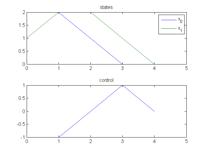
TomSym MPC example with TomSym.

This page is part of the TomSym Manual. See TomSym Manual.

This is an example of MPC for a linear, time-invariant system, illustrating how to use sym2prob and setParameter with tomSym for repeatedly solving the same optimization problem.

Note: This example code contains two alternative ways of setting up the problem. If you use this code as a basis for your own MPC controller, then you should probalby delete the "if 0" statement, and only keep the "else" part.

Reference: The problem definition is taken from the "Standard MPC" example in the YALMIP documentaion by Johan Löfberg. http://users.isy.liu.se/johanl/yalmip/pmwiki.php?n=Examples.StandardMPC

% Model data
A = [2 -1;1 0];
B = [1;0];
nx = size(A,2); % Number of states
nu = size(B,2); % Number of inputs

% MPC data
Q = eye(2);
R = 1;
N = 4; % Number of time-steps

% Make the initial state a symbol, so that we can use it as a parameter
% later.
x0 = tom('x0',nx,1);

Problem Setup

This example shows two ways of setting up the model. Change "if 0" to "if 1" to try the other one.

if 0
    % The more intuitive way to write the model involves a for-loop:

    u = cell(N,1); % Preallocate empty cell array.
    constraints = cell(N,1);

    objective = 0;
    x = x0;

    for k = 1:N
        u{k} = tom(['u' num2str(k)], nu, 1);

        % The symbolic expressions for x and the objective will grow inside
        % the loop, so at the last iteration, they will be quite large.
        % Remove the semicolons from the following lines to see how the
        % expressions grow.
        x = A*x + B*u{k};
        objective = objective + norm(Q*x,1) + norm(R*u{k},1);

        constraints{k} = { -1 <= u{k} <= 1, -5 <= x <=5 };
    end
else
    % A better way to solve the same problem:

    % Making all x(k) a decsion variables is numerically more sound, even
    % though it makes the number of unknowns larger.
    x = tom('x',nx,N);

    % Make the first column of u a separate symbol for compatibility with
    % the above variation of the code.
    u1 = tom('u1',nu,1);
    uk = tom('uk',nu,N-1);
    u = [u1 uk];

    % Matrix-matrix multiplication is equivalent to looping over the
    % columns of the second matrix and doing matrix-vector multiplication.
    constraints = {
        x == A*[x0 x(:,1:N-1)] + B*u
        -1 <= u <= 1
        -5 <= x <= 5
        };

    objective = sum(vec(abs(Q*x))) + sum(vec(abs(R*u)));
end

Compile the sybolic problem into a Prob structure

[objective, constraints] = rewriteV(objective, constraints);
ptype = tomDiagnose(objective, constraints);
Prob = sym2prob(ptype, objective, constraints);

Simulate a trajectory

Now that a Prob structure has been created, we can run the optimizatino multiple times without the overhead of processing symbols.

Ns = 5; % Number of steps to simulate
xt = zeros(nx,Ns+1);
xt(:,1) = [2;1];
ut = zeros(nu,Ns);
for i = 1:Ns
    Prob = setParameter(Prob, x0 == xt(:,i));
    Result = tomRun('snopt',Prob,0);
    solution = getSolution(Result);
    ut(:,i) = solution.u1;
    xt(:,i+1) = A*xt(:,i) + B*ut(:,i);
end

subplot(2,1,1);
plot(0:Ns,xt');
title('states');
legend({'x_0','x_1'});

subplot(2,1,2);
plot(0:Ns,[ut NaN(nu,1)]');
title('control');

Get rid of any temporary m-files created.

This example results in a linear programming, so no m-files are created. Cleanup is therefore striclty not needed, but we include it in case we want to modify the code to use a nonlinear model later. (Remove these lines if you want to keep the Prob structure after the script has finished.)

tomCleanup(Prob)
clear Prob