PROPT Multiphase Aircraft Trajectory Planning Example

This page is part of the PROPT Manual. See PROPT Manual.

This is an example of how to set up a multi-phase problem with PROPT.

% Copyright (c) 2010 by Tomlab Optimization Inc.

Problem description

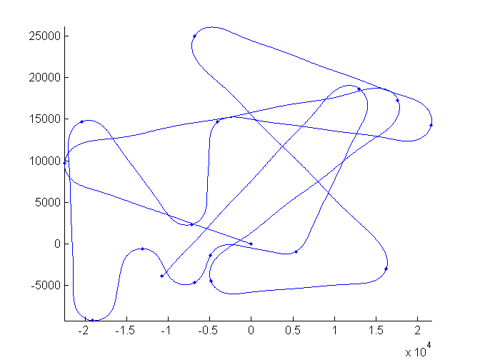
An airplne will fly through a given set of waypoints (in order) minimizing the distance flown, under constraints on the turning radius, and the rate at which it rolls in and out of turns.

The coordinate system is on the surface of the earth, which means that scale-factors change with latitude, and this must be included in the calcualtions.

% When setting up the problem, each leg of the trajectory is one PROPT
% phase. There are a total of 16 phases used.
%
% The phases are created inside of a for-loop. All states and controls are
% also created for each phase inside the for loop.

Constants

V=200;                  % velocity
dt=0.5;                 % time sampling (for plots)
g=9.81;                 % gravity acceleration
n=2;                    % load factor
R=V^2/(g*sqrt(n^2-1));  % minimum curvatre radius
Umax=V/R;               % Limit on angular velocity
udotmax = 0.01;         % Limit on rate-of-change of angular velocity

% Waypoints lat/long (generated at random)
WP = 0.02*[...
       0         0
  -10.15    4.37
    7.97    7.77
   -2.19   -2.00
    7.34   -1.33
   -3.07   11.23
    9.78    6.41
   -1.82    6.60
   -3.24    1.06
   -9.21    6.61
   -8.63   -4.14
   -5.91   -0.25
   -3.07   -2.07
   -2.23   -0.63
    2.42   -0.41
    5.86    8.38
   -4.86   -1.75]';
WP= (pi/180)*WP; % Convert from degrees to radians.
nWP=size(WP,2);

% Earth shape constants (Reference: WGS84)
a = 6378137.0; % semi-major axis [meters]
flinv = 298.257223563; % inverse flattening
b = a*(1-1/flinv); % semi-minor axis

% Meridional radius of curvature (Reference: Wikipedia)
rm = @(phi) (a.^2.*b.^2)./((a.*cos(phi)).^2+(b.*sin(phi)).^2).^(3/2);
% Normal radius of curvature
rn = @(phi) a^2./sqrt((a.*cos(phi)).^2+(b.*sin(phi)).^2);

Problem setup

np = 10; % Points per phase.

t = tom('t');

con = cell(1,nWP-1);
guess = cell(1,nWP-1);
tsum = 0;
td = cell(1,nWP-1);
p = cell(1,nWP-1);
x = cell(1,nWP-1);
y = cell(1,nWP-1);
heading = cell(1,nWP-1);
u = cell(1,nWP-1);

udot2sum = 0;

for i=1:nWP-1
    % For each leg we create a separate phase and unknowns
    td{i} = tom(['td' num2str(i)]);
    p{i} = tomPhase(['p' num2str(i)],t,tsum,td{i},np);
    setPhase(p{i}) % Needed so that we can use dot() without specifying the phase.
    x{i} = tomState(p{i}, ['x' num2str(i)]);
    y{i} = tomState(p{i}, ['y' num2str(i)]);
    heading{i} = tomState(p{i}, ['heading' num2str(i)]);
    u{i} = tomState(p{i}, ['u' num2str(i)]);

    con{i} = {
        initial(p{i},x{i}) == WP(1,i)
        initial(p{i},y{i}) == WP(2,i)
        final(p{i},x{i}) == WP(1,i+1)
        final(p{i},y{i}) == WP(2,i+1)
        collocate(p{i},dot(x{i}) == V*cos(heading{i})./rm(x{i}))
        collocate(p{i},dot(y{i}) == V*sin(heading{i})./(rn(x{i}).*cos(x{i})))
        collocate(p{i},dot(heading{i}) == u{i})
        mcollocate(p{i},-Umax <= u{i} <= Umax)
        mcollocate(p{i},-udotmax <= dot(u{i}) <= udotmax)
        };

    if i>=2
        % Continuity constraint for heading and u.
        % x and y are already continuous, because connect the waypoints
		%
        % The continuity constraint for the heading is mod 2*pi, which we
        % handle using the mod() function, centering around pi, rather than
        % making this a mixed-integer problem.
        con{i} = {con{i}
            mod(final(p{i-1},heading{i-1})-initial(p{i},heading{i})+pi,2*pi) == pi
            final(p{i-1},u{i-1}) == initial(p{i},u{i})
            };
    end

    dx0 = (WP(1,i+1)-WP(1,i))*rm(WP(1,i));
    dy0 = (WP(2,i+1)-WP(2,i))*rn(WP(1,i))*cos(WP(1,i));
    psi0 = atan2(dy0, dx0);
    td0 = sqrt(dx0^2+dy0^2)/V;

    guess{i} = {
        td{i} == td0;
        icollocate(p{i}, heading{i}==psi0 )
        icollocate(p{i}, u{i}==0 )
        icollocate(p{i}, x{i} == WP(1,i)+(WP(1,i+1)-WP(1,i))*(t-tsum)/td0)
        icollocate(p{i}, y{i} == WP(2,i)+(WP(2,i+1)-WP(2,i))*(t-tsum)/td0)
        };

    tsum = tsum + td{i};
    udot2sum = udot2sum + integrate(p{i}, dot(u{i})^2);
end

% Including a small penalty for dot(u)^2 in the objective yields a smoother
% trajectory.
obj = tsum + 100*udot2sum;

Call the solver

solution = ezsolve(obj,con,guess);

Problem type appears to be: con
Time for symbolic processing: 7.7262 seconds
Starting numeric solver
===== * * * =================================================================== * * *
TOMLAB - TOMLAB Development license  999007. Valid to 2011-12-31
=====================================================================================
Problem: ---  1: Problem 1                      f_k    1846.542685406830300000
                                       sum(|constr|)      0.000035431425208725
                              f(x_k) + sum(|constr|)   1846.542720838255500000
                                              f(x_0)   1752.077215102110600000

Solver: snopt.  EXIT=0.  INFORM=1.
SNOPT 7.2-5 NLP code
Optimality conditions satisfied

FuncEv   69 GradEv   67 ConstrEv   67 ConJacEv   67 Iter   58 MinorIter 5030
CPU time: 2.106014 sec. Elapsed time: 2.100000 sec. 

Make plot

% Interpolate the computed trajectory with even time-steps.
t_plot = 0:dt:subs(tsum,solution);
x_plot = zeros(size(t_plot));
y_plot = zeros(size(t_plot));
psiplot = zeros(size(t_plot));
u_plot = zeros(size(t_plot));
% Loop over phases, and interpolate for each phase.
for i=1:nWP-1
    ti = subs(initial(p{i},t),solution);
    t_f = subs(final(p{i},t),solution);
    ix = find(t_plot>=ti & t_plot<=t_f);
    % ix is the indexes of all points that lie in the current phase.
    x_plot(ix) = atPoints(p{i},t_plot(ix),subs(x{i},solution));
    y_plot(ix) = atPoints(p{i},t_plot(ix),subs(y{i},solution));
    psiplot(ix) = atPoints(p{i},t_plot(ix),subs(heading{i},solution));
    u_plot(ix) = atPoints(p{i},t_plot(ix),subs(u{i},solution));
end

% Plot the trajectory
clf
hold on
plot(rm(WP(1,1))*x_plot,rn(WP(1,1))*cos(WP(1,1))*y_plot) % Trajectory (scaled to meters)
hold on
plot(rm(WP(1,1))*WP(1,:),rn(WP(1,1))*cos(WP(1,1))*WP(2,:),'.') % Waypoints
hold off
axis image