TomSym compared to the Symbolic Toolbox

A hydroelectric dam.

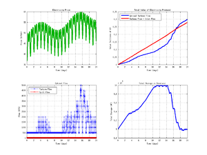
We look at the optimization problem of maximizing the revenue of a hydroelectric dam. This problem was published by By Seth DeLand of the MathWorks, as an example of how to combine their optimization and symbolic toolboxes. [1] We solve the same probem using tomSym and the TOMLAB solvers, noting a XXX times speed up. The problem can be solved in seconds with TOMLAB, as compared to hours with the MathWork's toolboxes.

Problem description

The dynamics of the dam is described by the following equations.

Electricity(t) = TurbineFlow(t-1)*[½ k1(Storage(t) + Storage(t-1)) + k2]

Storage(t) = Storage(t-1) + ∆t * [inFlow(t-1) - spillFlow(t-1) - turbineFlow(t-1)]

The problem is to maximize revenue (electricity times price), subject to the following constraints:

• 0 < Turbine Flow < 25,000 CFS
• 0 < Spill Flow
• Max change in Turbine and Spill Flow < 500 CFS
• Combined Turbine and Spill Flow > 500 CFS
• 50000 < Reservoir Storage < 100000 Acre-Feet
• The final reservoir level must equal the initial level (90000 AF)

The actual data used by DeLand can be downloaded from Matlab Central.[2]

tomSym code

To avoid attaching data files to our example, we will use an approximation to this data, as generated by the following Matlab code:

N = 480;
t = (0:N-1)';
inFlow = reshape(repmat(10*(107+[0 0 0 -3 3 2 2 -8 9 5 0 1 -6 -4 5 0 -6 -6 -17 -7]),24,1),N,1);
price = 46 + t./57 - 3*cos((t+46)/43) - 4*sin(pi/12*(t+4)) - 4*sin(pi/6*(t+1));

(The timing tests were run using both the original and the approximated data. Changes in indata has random effects on the number of iterations needed for convergence, but the effects are much smaller than the systematic differences between solvers.)

A few other consants are defined by DeLand as follows:

stor0 = 90000; % initial vol. of water stored in the reservoir (Acre-Feet)

k1 = 0.00003; % K-factor coefficient
k2 = 9; % K-factor offset

MW2kW = 1000; % MW to kW
C2A = 1.98347/24; % Convert from CFS to AF/HR

One the input data is defined, this is the entire code used to set up and solve the problem with TOMLAB:

turbineFlow = tom('turbineFlow',N,1);
spillFlow = tom('spillFlow',N,1);

outFlow = turbineFlow + spillFlow;

storage = stor0 + C2A*cumsum(inFlow - outFlow);

electricity = turbineFlow.*(0.5*k1*(storage + [stor0; storage(1:end-1)]) + k2)./MW2kW;

revenue = price*electricity; 

objective = -revenue; % Minimization objective

constraints = {
    0 <= turbineFlow <= 25000
    0 <= spillFlow
    -500 <= diff(outFlow) <= 500
    outFlow >= 500
    50000 <= storage <= 100000
    storage(end) == stor0
    };

guess = [];
 
options = struct;
options.solver = 'snopt';
options.scale = 'auto'

solution = ezsolve(objective, constraints, guess, options);

Solution

Plots of the result, when the approximate indata is used.

Although the Hessian is numeric this is not a quadratic programming. The Hessian is not positive semidefinite, and the objective is therefore not convex. There may exist local optima that are not as good as the global one. For this reason, the QP solvers in the TOMLAB suite return error messages, and a nonlinear solver had to be used instead.

The solution for the approximate input data is very similar to the one presented by DeLand. With identical input data, the solutions are of course nearly identical. (The TOMLAB solvers give a slightly worse objective value due to better constraint adherence.)

Timing measurments

In order to compare TOMLAB to the Mathworks' toolboxes, we ran a series of tests, using different problem sizes. Each test was run 5 times, and the mean of the middle 3 results was used.

Time for symbolic processing

Number of variables	Symbolic TB	tomSym
10	0.698 s	0.502 s
50	12.86 s	0.502 s
100	67.49 s	0.518 s
150	237.0 s	0.564 s

The time for deriving the Hessian using the symbolic toolbox increased approximately as N^2.7 as the number of variables increased. With tomSym, on the other hand, the time remained approximately constant.

Time for numeric solver

Number of variables	quadprog	KNITRO
10	0.0162 s	0.0165 s
50	0.0452 s	0.0318 s
100	0.2015 s	0.0829 s
150	0.4756 s	0.1847 s

KNITRO is about the same speed as quadprog on the smallest problem sizes, and about 2.5 times faster for larger problems. In every case, the time for the numeric solver is much smaller than the time for symbolic processing for problems this small.

Comparing tomSym to the symbolic toolbox

The main reason why tomSym is so much faster than the symbolic toolbox is that it can handle vector and matrix symbols. This means that matrix expressions are handled at approximately the same speed, regardless of the sizes of the symbolic matrices involved.

The symbolic toolbox, on the other hand, only handles scalar symbols. This means that both the number of expressions and their sizes increase as the size of symbolic matrices increase. The matlab code generated by the symbolic toolbox also becomes quite lengthy because of the use of multiple scalar operations instead of vector/matrix operations.

Footnote

The above code passes the same Hessian to the solver as DeLand's code. It is possible to get a much sparser Hessian, by making the water level a decision variable instead of a symbolic expression. All we need to do is to replace the previous expression for "storage" by a symbol definition:

    storage = tom('storage',N,1);

and then add one constraint

    constraints{end+1} = ( storage == [stor0; storage(1:N-1)] + inFlow - outFlow );