TomSym compared to the Symbolic Toolbox: Difference between revisions
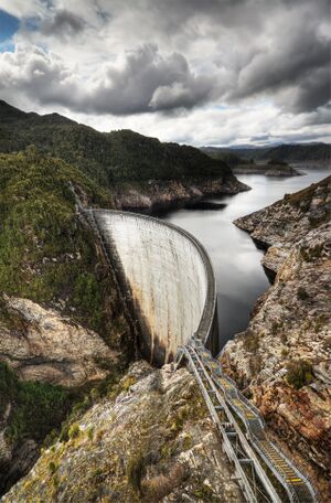
(Created page with "thumb|A hydroelectric dam. We look at the optimization problem of maximizing the revenue of a hydroelectric dam. This problem was published by By Seth De...") |
No edit summary |
||
| Line 8: | Line 8: | ||
Electricity(t) = TurbineFlow(t-1)*[½ k1(Storage(t) + Storage(t-1)) + k2] | Electricity(t) = TurbineFlow(t-1)*[½ k1(Storage(t) + Storage(t-1)) + k2] | ||
Storage(t) = Storage(t-1) + ∆t * [inFlow(t-1) - spillFlow(t-1) - turbineFlow(t-1)] | Storage(t) = Storage(t-1) + ∆t * [inFlow(t-1) - spillFlow(t-1) - turbineFlow(t-1)] | ||
The actual data used by DeLand can be downloaded from Matlab Central.[http://www.mathworks.com/matlabcentral/fileexchange/35856-optimization-in-matlab-an-introduction-to-quadratic-programming] | The actual data used by DeLand can be downloaded from Matlab Central.[http://www.mathworks.com/matlabcentral/fileexchange/35856-optimization-in-matlab-an-introduction-to-quadratic-programming] | ||
To avoid attaching data files to our example, we will use an approximation to this data, as generated by the following Matlab code: | To avoid attaching data files to our example, we will use an approximation to this data, as generated by the following Matlab code: | ||
< | <source lang="matlab"> | ||
N = 480; | |||
t = (0:N-1)'; | |||
inFlow = reshape(repmat(10*(107+[0 0 0 -3 3 2 2 -8 9 5 0 1 -6 -4 5 0 -6 -6 -17 -7]),24,1),N,1); | |||
price = 46 + t./57 - 3*cos((t+46)/43) - 4*sin(pi/12*(t+4)) - 4*sin(pi/6*(t+1)); | |||
</code> | </source> | ||
(The timing tests were run using both the original and the approximated data. There was no detectable difference in runtimes.) | |||
A few other consants are defined by DeLand as follows: | |||
<source lang="matlab"> | |||
stor0 = 90000; % initial vol. of water stored in the reservoir (Acre-Feet) | |||
k1 = 0.00003; % K-factor coefficient | |||
k2 = 9; % K-factor offset | |||
MW2kW = 1000; % MW to kW | |||
C2A = 1.98347/24; % Convert from CFS to AF/HR | |||
</source> | |||
One the input data is defined, this is the entire code used to set up and solve the problem with TOMLAB: | |||
<source lang="matlab"> | |||
turbineFlow = tom('turbineFlow',N,1); | |||
spillFlow = tom('spillFlow',N,1); | |||
outFlow = turbineFlow + spillFlow; | |||
storage = stor0 + cumsum(inFlow - outFlow); | |||
electricity = turbineFlow.*(0.5*k1*(storage + [stor0; storage(1:end-1)]) + k2); | |||
revenue = price*electricity; | |||
objective = -revenue; % Minimization objective | |||
constraints = { | |||
0 <= turbineFlow <= 25000 | |||
0 <= spillFlow | |||
-500 <= diff(outFlow) <= 500 | |||
outFlow >= 500 | |||
50000 <= storage <= 100000 | |||
storage(end) == stor0 | |||
}; | |||
guess = []; | |||
options = struct; | |||
options.solver = 'snopt'; | |||
solution = ezsolve(objective, constraints, guess, options); | |||
</source> | |||
Revision as of 11:46, 20 November 2013
We look at the optimization problem of maximizing the revenue of a hydroelectric dam. This problem was published by By Seth DeLand of the MathWorks, as an example of how to combine their optimization and symbolic toolboxes. [1] We solve the same probem using tomSym and the TOMLAB solvers, noting a XXX times speed up. The problem can be solved in seconds with TOMLAB, as compared to hours with the MathWork's toolboxes.
The dynamics of the dam is described by the following equations.
Electricity(t) = TurbineFlow(t-1)*[½ k1(Storage(t) + Storage(t-1)) + k2]
Storage(t) = Storage(t-1) + ∆t * [inFlow(t-1) - spillFlow(t-1) - turbineFlow(t-1)]
The actual data used by DeLand can be downloaded from Matlab Central.[2] To avoid attaching data files to our example, we will use an approximation to this data, as generated by the following Matlab code:
N = 480;
t = (0:N-1)';
inFlow = reshape(repmat(10*(107+[0 0 0 -3 3 2 2 -8 9 5 0 1 -6 -4 5 0 -6 -6 -17 -7]),24,1),N,1);
price = 46 + t./57 - 3*cos((t+46)/43) - 4*sin(pi/12*(t+4)) - 4*sin(pi/6*(t+1));
(The timing tests were run using both the original and the approximated data. There was no detectable difference in runtimes.)
A few other consants are defined by DeLand as follows:
stor0 = 90000; % initial vol. of water stored in the reservoir (Acre-Feet)

k1 = 0.00003; % K-factor coefficient
k2 = 9; % K-factor offset

MW2kW = 1000; % MW to kW
C2A = 1.98347/24; % Convert from CFS to AF/HR
One the input data is defined, this is the entire code used to set up and solve the problem with TOMLAB:
turbineFlow = tom('turbineFlow',N,1);
spillFlow = tom('spillFlow',N,1);

outFlow = turbineFlow + spillFlow;

storage = stor0 + cumsum(inFlow - outFlow);

electricity = turbineFlow.*(0.5*k1*(storage + [stor0; storage(1:end-1)]) + k2);

revenue = price*electricity;

objective = -revenue; % Minimization objective

constraints = {
    0 <= turbineFlow <= 25000
    0 <= spillFlow
    -500 <= diff(outFlow) <= 500
    outFlow >= 500
    50000 <= storage <= 100000
    storage(end) == stor0
    };

guess = [];

options = struct;
options.solver = 'snopt';

solution = ezsolve(objective, constraints, guess, options);